One-pot recipe for small polaron localisation

August 4, 2020

When an excess charge (electron or hole) is added to a perfect crystal, there are several possible scenarios. In dielectric materials, the two extremes are a large polaron (wave function extending over many unit cells) and small polarons (wave function localised in a single unit cell; often on one atom). Austin and Mott provided an essential overview of the topic in 1969.

I received several recent queries on this topic, so I thought it may be best to write a short post... I won't discuss large polarons here; a good place to start for those is the PolaronMobility.jl package and related reading (e.g. the work of Dan Davies on rapid descriptors).

Ingredients

An electronic structure approach such as DFT that includes reliable atomic forces, e.g. GW theory won't necessarily help you here

An exchange-correlation functional without severe self-interaction errors, e.g. bare LDA/GGA are often insufficient to describe small polarons, hybrid functionals can be better (sensitive to % HF exchange), DFT+U can be okay (sensitive to choice of U)

A crystal where small polarons form. Experimental evidence is often present from photoemission, EPR, conductivity measurements, etc.

Method

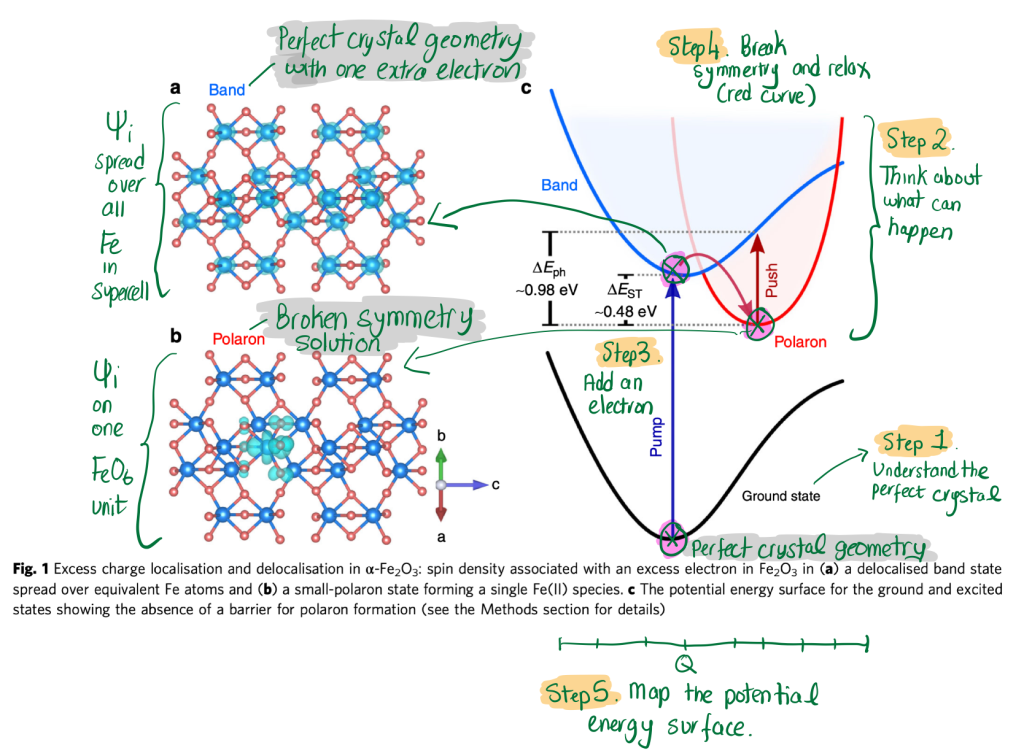
I will take the example of Fe₂O₃, which we tackled in collaboration with pump-push-probe spectroscopy led by Artem Bakulin. I give my approach for dealing with an excess electron, but many others exist, so don't take this as gospel.

1. Understand the perfect crystal. In Fe₂O₃, the formal ions present are Fe(III), which have a d⁵ electronic configuration in roughly octahedral coordination. These d⁵ electrons prefer to be in a high spin configuration, and the lowest energy solution of the crystal is layer-by-layer anti-ferromagnetism along the hexagonal (0001) axis [1].
2. Think about what can happen. Adding an electron to Fe₂O₃ is likely to reduce Fe from Fe(III) d⁵ to Fe(II) d⁶. The d⁶ configuration in an octahedral field can be high spin or low spin, so we'll have to check both solutions to find the lowest in total energy.
3. Add an electron and check the result. I take a supercell of my perfect crystal and change the electron count by 1. In this case, I find that the excess electron is delocalised across all equivalent Fe sites. I call this a "band electron" and it provides a useful reference energy.
4. Break symmetry and relax the ions. Often local optimisers fail to break the crystal symmetry spontaneously, so you have to give a "push" and then fall into the closet local minimum. There are several approaches to do this, such as: (a) replacing one Fe by another ion with appropriate radius, relaxing, and then substituting Fe back in; (b) adding small random atomic displacements around one Fe in the supercell; (c) a selective distortion around one Fe. Following geometry optimisation, they should all arrive at the same solution but may require different amounts of computer time. This is discussed in detail in the recent paper of Pham and Deskins. Here the symmetry breaking and atomic relaxation serve to localise the excess electron and I call this a "small polaron".
5. Map out the potential energy surface. So far we have two points, which is sufficient to define a polaron binding energy, but we can do more. The atomic geometries of the perfect crystal and the localised polaron can be used to define a configurational coordinate Q that maps between them (e.g. there are relevant scripts in CarrierCapture.jl). The challenge is over what range it is possible to obtain the band / polaron solutions. This requires playing with the wavefunction initialisation in whatever code you are using. A hands-on approach would be using full occupation control or constrained DFT. This is the direction we are actively working on, so I'll have to save that icing for later...

[1] I incorrectly commented that the layer-by-layer AFM description was only possible in the hexagonal setting of Fe₂O₃. Nicola Spaldin correctly pointed out to me a few weeks ago that it is possible in the primitive trigonal cell.